Chapter 4 Analytical Approach

Using Indicators to Inform the Status of salmon Conservation Units and their Habitats

We apply a suite of indicators to assess both the biological and habitat status of salmon Conservation Units (CUs). Defined as “measures of pressures, states, and/or responses”, indicators depict the condition of species, habitats, and/or systems to improve one’s understanding of the linkages among drivers, stressors, conditions, and management actions (Nelitz et al. 2007). The indicators and approach that we use align with Strategies 1 and 2 of the Wild Salmon Policy (Fisheries and Oceans Canada 2005) that call for standardized assessment and monitoring of the salmon CUs and their freshwater habitats (Holt et al. 2009; Stalberg et al. 2009).

Relevant salmon indicators for informing population and habitat status have several criteria:

• They are measurable, relevant to the health and persistence of salmon as they characterize either key population dynamics or habitat conditions;
• The data are available over broad spatial and temporal scales;
• The data are updated consistently;
• The data have consistent collection protocols;
• The data are in a format that allows easy integration into PSF’s data systems;
• The indicators can be tracked over time;
• They can be used to inform management decisions for threatened or at-risk salmon CUs.

To quantify the suite of population and habitat status indicators that we use, we have continued to lead a major effort to compile and synthesize salmon-related data in each of the Regions where we operate. While a large amount of salmon-related data already exists, they are often not readily available, not well documented, and not compiled in a single location. Our efforts focus on bringing existing information together in a standardized format into a single, centralized location (i.e. the Salmon Data Library) and summarizing the data in valuable ways for monitoring and assessing salmon CUs and their habitats (i.e. the Pacific Salmon Explorer).

We then calculate and apply benchmarks for each indicator to assess status using a ‘stoplight’ approach. The result is a qualitative assessment of each indicator as either red, amber, or green, depending on the current data relative to a lower or upper benchmark (Figure 4.1). The intent is that decision-makers can then apply management measures to improve the status of a CU and/or salmon-bearing watershed, for example, from Red to Amber or Amber to Green (Fisheries and Oceans Canada 2005).

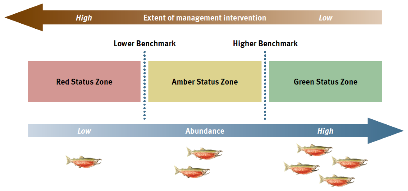
Figure 4.1: Benchmarks and biological status zones under the Wild Salmon Policy (DFO, 2005).

4.1 Population Status: Indicators & Benchmarks

To characterize key salmon population dynamics, temporal trends in fisheries data, and assess the biological status of salmon CUs across the Pacific Region, we compile and synthesize the following information:

• Spawner survey locations;
• Observed spawner counts in indicator and non-indicator streams;
• Juvenile surveys in streams;
• Estimates of spawner abundance at the CU-level;
• Estimates of total run size;
• U.S. and Canadian catch;
• Exploitation rate;
• Hatchery release data; and
• Recruits-per-spawner datasets.

The data sources and analyses differ among regions, with the main differences occurring between the North and Central Coast (Nass, Skeena, Central Coast Regions) and the South Coast (Fraser and Vancouver Island & Mainland Inlets Regions). Region-specific data nuances are included in Regions.

We synthesize the types of data listed above to generate output datasets that are available for download in the Salmon Data Library. These output datasets are visualized in the Pacific Salmon Explorer through nine population indicators. These datasets also inform a CU-level Hatchery Contribution Score and Data Quality Scores. The data compilation exercise also highlights data gaps across and within Regions. We aim to update these key datasets annually or as new input data become available.

4.1.1 Overview of Population Indicators

We use nine indicators to characterize the population status of each Conservation Unit in the Pacific Salmon Explorer.

1. Spawner Surveys
2. Juvenile Surveys
3. Hatchery Releases
4. Spawner Abundance
5. Run Timing
6. Catch and Run Size
7. Recruits-per-Spawner
8. Trends in Spawner Abundance
9. Biological Status

These indicators provide information on the current state of salmon CUs and trends over time. The first three indicators involve displaying stream-level information organized by CU. The last seven indicators involve synthesizing data at the CU-level, with the Hatchery Release indicator involving both the stream-level release data and a CU-level Hatchery Contribution Score. Here, we describe the general approach to compile and synthesize data for each of these population indicators. Detailed methods that depend on the specifics of the available data vary by Region and are documented in the Regions section.

4.1.1.1 Spawner Surveys

Spawner surveys show the observed numbers of spawning salmon of each species returning to specific streams each year. Spawner surveys provide a fundamental piece of information needed to assess the status of salmon CUs over time. In the Pacific Salmon Explorer we draw on spawner survey data from the New Salmon Escapement Database (NuSEDS) and other sources detailed in the region Regions section to visualize the spatial and temporal coverage of spawner surveys for each CU in the Pacific Salmon Explorer. The NuSEDS data requires substantial cleaning prior integration into the PSE due to inconsistencies in populations and locations names and identification numbers (see Appendix 2 for an exhaustive description of the cleaning procedure).

We distinguish spawner surveys in indicator streams and non-indicator streams for each species. Indicator streams are observed consistently in recent decades, tend to have high spawner abundance and to be monitored using intensive methods that provide greater accuracy. Therefore, indicator streams are understood to provide reliable indices of abundance and are assumed to be representative of returns to other streams nearby (English 2016). In comparison, non-indicator streams tend to have less consistent survey coverage, more variable survey methods, and/or may be more difficult to survey. A number of both indicator and non-indicator streams within a CU may be surveyed in a given year. On the Pacific Salmon Explorer, we use the indicator stream designation from LGL Ltd (English et al. 2018) for the North and Central Coast Regions (Skeena, Nass, and Central Coast), and from DFO (NuSEDS) for all other Regions.

A variety of methods are used to survey spawners in both indicator and non-indicator streams, and methods vary by species, CU, and stream. Spawner counts can be produced from a single visual survey of a stream by foot, by counting fish through a complete counting fence, or by aerial (helicopter) surveys. Survey methodology can also change over time according to changes in capacity and funding. For instance, some streams that were historically monitored by visual surveys on foot are now enumerated via a counting fence or aerial surveys. We account for these discrepancies in the survey methods by defining a Data Quality Score to each CU (see Data Quality section below).

For steelhead, we used spawner survey data from a variety of sources, depending on the Region. Steelhead monitoring data have not been maintained in a centralized database like NuSEDS, so we compiled and synthesized spawner survey data from disparate sources, including many monitoring projects led by the Province of BC. Streams with spawner survey data for steelhead have not been classified as indicator and non-indicator streams. Consequently, we provisionally classified all streams with available spawner survey data as indicator streams. More specific details on the specific sources of spawner survey data for steelhead are summarized by Region in the Regions section.

4.1.1.2 Juvenile Surveys

Estimates of juvenile abundance indicate the number of out-migrating smolts that were counted in a given year for each stream within a CU (where available) or for some steelhead CUs, the estimated density of juvenile steelhead in a stream for a given year. We also calculate the geometric mean of juvenile abundance or density as it is less sensitive to infrequent high abundance years.

4.1.1.3 Hatchery Releases

While salmon hatcheries play a role in the conservation and management of Pacific salmon, hatchery releases can also pose risks to wild salmon (McMillan et al. 2023). Juvenile hatchery fish can outcompete wild juveniles for limited food resources, and there is increasing evidence that high hatchery salmon abundance at sea is related to decreased wild salmon productivity due to limitations of ocean carrying capacity (Ruggerone and Irvine 2018; Connors et al. 2020). Hatchery-produced spawners can also interbreed with wild salmon, with implications for the genetic diversity and productivity of wild populations. Hatchery-produced fish can also exacerbate issues with mixed-stock fisheries, which can affect threatened or at-risk salmon populations.

Given these concerns and other potential impacts of hatcheries on wild salmon abundance and productivity, we visualize the number of fish released from specific locations under the hatchery releases indicator. For each hatchery facility (i.e. the facility where eggs are hatched), we show the name, years in use, and facility type. Hatchery operations range in size and production from small to large-scale, with different purposes. There are four types of hatcheries shown on the Pacific Salmon Explorer, as defined by Fisheries and Oceans Canada’s Salmon Enhancement Program (Table 4.1)

Hatchery facilities may release fish at one or more release sites. We show the locations and numbers of fish released through time at each of these release sites. Locations also include additional information: the name of the site, the years that site was in use, the type or life stage at which juvenile salmon were released, and the broodstock CU (CU from which the hatchery broodstock originates). Juvenile salmon are released at various life stages and under various hatchery practices (e.g. some juveniles are released in rivers as fed fry, while others are reared for longer in the hatchery and then transferred to a sea pen in the ocean, where they are eventually released) which can affect their survival (James et al. 2023). Pacific salmon data on hatchery locations, release sites, and release numbers were provided by DFO Salmon Enhancement Program staff. For steelhead, these data were accessed through the BC Data Catalogue. The information on hatchery releases in streams is also synthesized at the CU-level (see Hatchery Contribution Score, below).

Table 4.1: Types of hatcheries operated in BC and visualized on the Pacific Salmon Explorer.

Type of Hatchery	Description
Enhancement operations	Major hatcheries with high production
Community economic development	Smaller-scale community-based hatcheries
Designated public involvement	Similar to community economic development but smaller
Public involvement unit	Very small-scale hatcheries

4.1.1.4 Spawner Abundance

We visualize both observed and estimated spawner abundance on the Pacific Salmon Explorer. This indicator provides estimates of the total numbers of spawners that return to spawn each year for each CU. Observed spawner abundance is the sum of all spawner survey data as documented in NuSEDS, while estimated spawner abundance generally accounts for streams that are not surveyed in a given year by following expansion procedures. The approach for expanding from observed spawners to estimate the total spawners in a CU depends on the region and species, and are documented in the Regions section. Unless specified otherwise, estimated CU-level spawner abundance is used as input in the Catch and Run Size, Recruits-per-Spawner, and Trends in Spawner Abundance indicators described below and when assessing biological status for each CU (see Appendix 3).

4.1.1.5 Run Timing

Run timing represents the average time window over which adult salmon enter freshwater on their return migrations to spawn. Run timing is estimated using a range of methods, including test fisheries, daily counting at weirs, and expert judgment. We adjust run timing estimates based on the sampling location so that the run timing shown in the Pacific Salmon Explorer represents river entry timing regardless of where the data were collected. Specifically, data that are from test fisheries operating more than 100 km from the mouth of the river (e.g., Area 20 test fisheries for some Fraser CUs) or from sampling more than 1-day migration upstream are adjusted for the time it takes salmon to migration to/from the river mouth based on published estimates of migration speed by species. The methods for estimating run timing and approaches to compiling these data for specific CUs are detailed in the Regions chapter and in Wilson and Peacock (in prep.).

Where data are available, we show the estimated run timing for each CU as the relative proportion of the CU that is expected to enter freshwater on a given day averaged over all historical information for the CU. Often, daily counts are not available but there is information on the dates for start (2.5th percentile), peak (50th percentile), and end (2.5th percentile) run timing. In these cases, we assume a mixed normal distribution with different standard deviations for the left- and right-hand sides based on the start and end dates, respectively. If the end date or start date is missing, we assume equal tails. If only peak or start date is available, we assume a standard deviation equal to the average standard deviation among other CUs of the same region and species. If applied, these assumptions are reflected in the run timing data quality criteria (see Data Quality).

4.1.1.6 Catch & Run Size

Catch estimates report the number of adult salmon caught in commercial (including both Canadian and U.S.), recreational, and First Nations’ food, social, and ceremonial (FSC) fisheries. Run size refers to the number of adult salmon that return from the ocean in a given year, including both escapement (i.e. estimated spawner abundance) and those that are caught (i.e. catch) at a CU-level. The exploitation rate is calculated as the proportion of a given run caught in all fisheries. This indicator provides important information on the long-term harvest rate of each CU, which has implications for the number of salmon returning to spawning grounds over time.

4.1.1.7 Recruits-per-Spawner

Recruits-per-spawner estimates the number of adult salmon produced per spawner in the previous generation. This indicator provides valuable information on the recruitment of salmon within a CU when calculations are available over the long term. This can improve our understanding of survival within and among CUs. If the number of recruits-per-spawner is below one, the population will decline over time.

For species with variable age-at-return, estimating the number of recruits for a given brood year requires information on total run size (i.e. catch plus escapement) and the distribution of ages of returning fish over multiple years. Recruits-per-spawner is then calculated as the number of recruits divided by the number of spawners for each brood year, based on CU-level estimates of spawning abundance. This indicator is relatively data-intensive as it requires information on total run size, spawner abundance, and the ages of salmon returning to spawn.

4.1.1.8 Trends in Spawner Abundance

Trends in spawner abundance is an estimate of the average change in estimated spawner abundance at the CU-level. This indicator highlights long-term changes that could otherwise be masked by high interannual variability in spawner abundance.

When calculating trends, we take the natural logarithm of spawner abundance and smooth the time series using a one-generation moving average, which minimizes the impact of outliers (i.e. anomalously high or low abundance years) on the overall trend (D’Eon-Eggertson et al. 2015). We fit a linear model to estimate the slope in log-transformed, smoothed spawner abundance over time. When estimated spawner abundance is zero, which occurs for only a few years, we add a small number (0.01) before log-transforming and smoothing. Linear models are fitted to log-transformed, smoothed spawner abundance over the most recent three generations to estimate the short-term trend, and over all years of data to estimate the long-term trend.

We report the magnitude of the trend as the total percent change over the short-term and long-term from the model-predicted abundance. The total percent change for the short-term trend is calculated as: \[\left( \exp(m_{3G} * (3G -1)) - 1 \right)\times 100, \] where \(m_{3G}\) is the estimated slope over the most recent three generations and \(G\) is the generation length in years. We do not show the short-term trend if there are fewer than \(G\) years with estimated spawner abundance in the most recent three generations.

The total percent change for the long-term trend is calculated as: \[\left( \exp(m_{LT} * (Y_t - Y_0)) - 1 \right) \times 100,\] where \(m_{LT}\) is the estimated slope over all years of data, \(Y_0\) and \(Y_t\) are the oldest and most recent years in the time series, respectively (e.g. 1970 and 2022).

Assuming the data are reliable, the long-term trend is better at detecting true changes in abundance, enabling more appropriate management responses (Porszt et al. 2012; D’Eon-Eggertson et al. 2015).

4.1.1.9 Biological Status

The biological status assessments that we complete and visualize on the Pacific Salmon Explorer are guided by the approaches recommended under Strategy 1 of the Wild Salmon Policy (Fisheries and Oceans Canada 2005) and by (Holt et al. 2009), as well as additional recommendations from our independent Population Science Advisory Committee. Candidate benchmarks for evaluating the status of CUs have been proposed for four classes of indicators (Holt et al. 2009), which include:

1. Current spawner abundance;
2. Trends in spawner abundance over time;
3. Distribution of spawners within the CU; and
4. Fishing mortality relative to stock productivity.

We assess biological status using a metric of current spawner abundance, while providing information on other indicators where available. The assessment of biological status is more involved, and our approach to quantifying metrics and benchmarks is detailed in section Benchmarks for Assessing Biological Status.

4.1.2 Hatchery Contribution Score

Hatchery-produced salmon are released in streams throughout BC, resulting in salmon populations that are considered to be hatchery-produced to varying degrees. We assess and display the current Hatchery Contribution Score for salmon CUs based on a standardized approach that draws on the best available data for all spawning streams within CUs across BC. The Hatchery Contribution Score is an assessment of the extent of hatchery activity within a CU over the last two generations.

Table 4.2: Stream Hatchery Releases score categories for spawning streams.

Stream Enhancement Level	Definition
None	No records of enhancement
Low	No records of enhancement over the previous two generations
Moderate	Less than 25% enhancement over the previous two generations
High	More than 25% enhancement over the previous two generations
Not Assessed	The Enhancement Level for this Conservation Unit has not been assessed

The determination of a CU’s Hatchery Contribution Score begins with assessing the extent of hatchery influence among individual spawning streams (indicator and non-indicator) within that CU, based on methods developed by DFO (Brown et al. 2019; Brown et al. 2020). Assessments of stream-level hatchery influence may draw on three types of information: 1) the number of coded wire tags (CWT) recovered from spawners; 2) the number of juveniles released from hatcheries within the CU; and 3) the number of fish collected for broodstock. If CWT-based estimates are available, then we use the proportion of returning spawners that have CWTs to quantify stream-level hatchery influence. Otherwise, we use the highest number from either the number of juvenile releases or the number of collected broodstock. This information is used to assign a categorical assessment of stream-level hatchery influence (high, moderate, low, none, not assessed; Table 4.2). For example, if more than 25% of spawners have CWTs, or more than 25% of years have records of juvenile releases or broodstock collection, then the stream is ranked as having high hatchery influence (Table 4.2). Data on hatchery activities for each spawning stream for southern BC Chinook were provided by DFO (Brown et al. 2019; Brown et al. 2020). For other species and CUs, we assessed stream-level hatchery influence based on data provided by the DFO’s Salmon Enhancement Program. In contrast to Brown et al. (2019), we assessed stream-level hatchery influence over the most recent two generations in alignment with the definition of wild salmon under Canada’s Wild Salmon Policy.

To arrive at a CU-level Hatchery Contribution Score, we calculate the proportional contribution, \(c\), of spawners from streams with moderate or high stream-level hatchery influence to the total spawners in each CU: \[ c = \frac{\sum_{i \in H}{\bar{S}_i}}{\sum_{j = 1}^n{\bar{S}_j}}\]

where \(\bar{S_i}\) is the geometric mean number of spawners in stream \(i\) over the most recent two generations, \(H\) is the set of indices of streams that have moderate or high stream-level hatchery influence over the most recent two generations, and \(n\) is the total number of streams in the CU. The CU-level Hatchery Contribution Score is then assigned as none, low, moderate, or high based on the value of \(c\) (Table 4.3). Note that the distinction between none and low is related to the timeframe of hatchery releases, with a score of low indicating that there has been no records of hatchery influence (either returns of CWT spawners or releases of hatchery fish) in the most recent two generations but there are prior recrods of hatchery influence. The CU is assigned a score of not assessed if there is insufficient information to assess stream-level hatchery releases.

Table 4.3: CU Hatchery Contribution Scores, as generated based on the categories in Table 4.2 for individual spawning streams.

Hatchery Contribution Score	Definition
None	There are no records of hatchery releases in the CU
Low	There are no records of hatchery releases in the CU in the most recent two generations (\(c = 0\))
Moderate	Less than 25% of spawners within the CU are from streams with moderate or high hatchery influence (\(0 < c <0.25\))
High	At least 25% of spawners within the CU are from streams with moderate or high hatchery influence (\(c \geq 0.25\))
Not Assessed	There was insufficient information to assess stream-level hatchery influence for the CU

4.1.3 Data Quality Scores

The quality of data shown in the Pacific Salmon Explorer varies widely among Regions, species, CUs, and streams. For instance, spawner abundance obtained from a single aerial survey is less reliable than counts obtained from an unbroken counting fence. We combine spawner survey data with other datasets, such as catch, to determine total run size and to assess the biological status of CUs. The data quality for each of these data types is important to consider when interpreting the population indicators shown in the Pacific Salmon Explorer.

We developed a standardized approach to assess the quality of data used to estimate populations indicators for each CU based on one or more of seven data quality criteria (Table 4.4). We assign scores of 1-5 to each of these four criteria and present the average score across relevant criteria as the Data Quality Score (\(Q\)) for each population indicator and CU. Numeric scores are translated to categorical data quality outcomes of low (\(1 \leq Q < 1.5\)), low-medium (\(1.5 \leq Q < 2.5\)), medium (\(2.5 \leq Q < 3.5\)), medium-high (\(3.5 \leq Q < 4.5\)), and high (\(4.5 \leq Q \leq 5\)). A score of zero means that there were no data for that CU..

Table 4.4: Summary of the seven criteria used to score overall CU-level data quality for population indicators.

Data quality criteria	Definition	Relevant population indicator(s)
Spawner survey method	The quality of spawner survey data, based on the survey methods used across all indicator streams within the CU over the most recent generation.	Spawner surveys, spawner abundance, recruits-per-spawner, trends in spawner abundance, biological status
Spawner survey coverage	How representative spawner surveys are of the CU, measured as the proportion of total spawners in the CU that spawn in indicator streams.	Spawner abundance, recruits-per-spawner, trends in spawner abundance, biological status
Spawner survey execution	How consistently indicator streams have been monitored, measured as the proportion of indicator streams that were surveyed in the most recent generation.	Spawner abundance, recruits-per-spawner, trends in spawner abundance, biological status
Juvenile survey method	The quality of juvenile survey data, based on the survey methods used across all years and locations of juvenile surveys in the CU.	Juvenile surveys
Run timing quality	The quality of run timing data, based on the number of years of data, the currency of the data, and whether sampling captured the entirety of the run.	Run timing
Catch estimation method	The quality of catch estimates for the CU based on a qualitative assessment of the rigor of the catch estimation method.	Catch and run size, recruits-per-spawner, biological status
Stock ID	The quality of recent stock identification data used in catch estimation for the CU.	Catch and run size, recruits-per-spawner, biological status

4.1.3.1 Spawner Survey Method

This criterion indicates the quality of spawner survey data over the most recent generation, based on the survey methods and sampling effort across all indicator streams within the CU. The CU-level spawner survey method data quality criteria is calculated as the average of stream-level data quality scores across all indicator streams (as defined by DFO) within the CU. We only quantify data quality for indicator streams because these are the streams that are typically used in expansion and infilling procedures to generate CU-level spawner abundances, while data for non-indicator streams are not directly used.

The stream-level data quality scores that we use to calculate a CU-level spawner survey method score are recorded by DFO in the NuSEDS database for each population and year. DFO measures stream-level survey quality on a six-point scale based on a standardized scoring rubric (Table 4.5) based on survey methodology and effort. These stream-level data quality scores reflect the highly variable spawner abundance data within and across spawning streams, which arises largely from differences in spawner survey methodology. To improve the communication of the stream-level data quality scores, we translate the “Estimate Classification Type” provided by DFO in NuSEDS into categories labeled as Unknown, Low, Medium-Low, Medium, Medium-High, and High (Table 4.5).

Table 4.5: Stream Survey Quality Criteria for the Estimate Classification field in NuSEDS (provided by Bruce Baxter, DFO), showing our categories in the “Data Quality Score on the Pacific Salmon Explorer” column.

Data Quality Score on the Pacific Salmon Explorer	Estimate Type	Survey Method(s)	Reliability (within stock comparisons)	Units	Accuracy	Precision
High	1: True Abundance, high resolution	Total, seasonal counts through fence or fishway; virtually no bypass	Reliable resolution of between year differences >10% (in absolute units)	Absolute abundance	Actual, very high	Infinite (i.e. + or - 0%)
Medium-High	2: True Abundance, medium resolution	High effort (5 or more trips), standard methods (e.g. mark-recapture, serial counts for area under the curve, etc.)	Reliable resolution of between year differences >25% (in absolute units)	Absolute abundance	Actual or assigned estimate and high	Actual estimate, high to moderate
Medium	3: Relative Abundance, high resolution	High effort (5 or more trips), standard methods (e.g. equal effort surveys executed by walk, swim, overflight, etc.)	Reliable resolution of between year differences >25% (in absolute units)	Relative abundance linked to method	Assigned range and medium to high	Assigned estimate, medium to high
Medium-Low	4: Relative Abundance, medium resolution	Low to moderate effort (1-4 trips), known survey method	Reliable resolution of between year differences >200% (in relative units)	Relative abundance linked to method	Unknown assumed fairly constant	Unknown assumed fairly constant
Low	5: Relative Abundance, low resolution	Low effort (e.g. 1 trip), use of vaguely defined, inconsistent, or poorly executed methods	Uncertain numeric comparisons, but high reliability for presence or absence	Relative abundance, but vague or no i.d. on method	Unknown assumed highly variable	Unknown assumed highly variable
Low	6: Presence or Absence	Any of above	Moderate to high reliability for presence/absence	(+) or (-)	Medium to high	Unknown
Unknown	Unknown	Unknown	Unknown	Unknown	Unknown	Unknown

To determine CU-level spawner survey method criteria, we calculate a weighted average of the stream-level survey method data quality scores across all indicator streams over the most recent generation within the CU (Table 4.6). The average survey method score over the most recent generation for each stream is weighted by the geometric average spawner abundance of that survey stream over the sum of the average spawner abundances to all indicator streams in the CU. Where there are known issues with DFO’s indicator stream list in NuSEDS, we manually override those data quality scores and substitute expert derived assessments of data quality based on expert knowledge of spawner survey methods. Specifically, this includes streams on the north and central coast (English 2016) and southern BC Chinook (Brown et al. 2020). We do not include survey years where spawner survey methods are Unknown in the survey method scores. Note that this score reflects the reliability of the estimates of current spawner abundance for a CU over the most recent generation and not the reliability of estimates across the entire time series.

Table 4.6: CU-level Survey Quality scores. Q = CU-level survey quality score (the weighted average of the stream-level survey method data quality values for all indicator streams over the most recent generation).

Score	Definition
0 - Not applicable	No spawner surveys were completed for this Conservation Unit over the most recent generation.
1 - Low	4.5 < Q < 6. Most of the spawner surveys were performed with low-effort or inconsistently executed methods, resulting in variable accuracy and precision.
2 - Medium-Low	3.5 < Q < 4.5. Most of the spawner surveys were performed with medium to low effort, using methods such as a stream walk, swim, or overhead flight, resulting in unknown accuracy and precision.
3 - Medium	2.5 < Q < 3.5. Most of the spawner surveys were performed with high effort, using methods such as a stream walk, swim, or overhead flight, resulting in medium to high accuracy and precision.
4 - Medium-High	1.5 < Q < 2.5. Most of the spawner surveys were performed with high effort, using methods such as mark-recapture, resulting in medium to high accuracy and precision.
5 - High	1 < Q < 1.5. Most of the spawner surveys produce counts of total spawners, using methods such as a fence or fishway, resulting in very high accuracy and precision.

4.1.3.2 Spawner Survey Coverage

This score is calculated from the proportion of observed spawners in the CU that are counted in indicator streams. We then translate the spawner survey coverage score into a scale of 0-5 (labeled as Not Applicable, Low, Medium-Low, Medium, Medium-High, and High; Table 4.7).

Table 4.7: Spawner survey coverage scores.

Score	Definition
0 - Not applicable	No spawner surveys were completed for this Conservation Unit.
1 - Low	1-30% of spawners within the Conservation Unit are represented by indicator streams.
2 - Medium-Low	30-49% of spawners within the Conservation Unit are represented by indicator streams.
3 - Medium	50-69% of spawners within the Conservation Unit are represented by indicator streams.
4 - Medium- High	70-89% of spawners within the Conservation Unit are represented by indicator streams.
5 - High	90-100% of spawners within the Conservation Unit are represented by indicator streams.

4.1.3.3 Spawner Survey Execution

This criterion indicates how consistently indicator streams in the CU have been surveyed over the most recent generation, measured as the proportion of indicator streams that have data in the most recent generation. To calculate Spawner Survey Execution, we calculate the average proportion of indicator streams that are surveyed within the CU in each year of the most recent generation. We then translate the proportion into a scale of 0-5 (labeled as Not Applicable, Low, Medium-Low, Medium, Medium-High, and High; Table 4.8).

Table 4.8: Spawner survey execution scores.

Score	Definition
0 - Not applicable	No surveys were completed for this Conservation Unit over the most recent generation.
1 - Low	1-20% of all indicator streams in the Conservation Unit were surveyed each year in the most recent generation.
2 - Medium-Low	21-40% of all indicator streams in the Conservation Unit were surveyed each year in the most recent generation.
3 - Medium	41-60% of all indicator streams in the Conservation Unit were surveyed each year in the most recent generation.
4 - Medium-High	61-80% of indicator streams in the Conservation Unit were surveyed each year over the most recent generation.
5 - High	81-100% of all indicator streams in the Conservation Unit were surveyed each year in the most recent generation.

4.1.3.4 Juvenile Survey Method

This criterion indicates the quality of the juvenile survey data based on the survey approach as outlined in Table 4.9. The CU-level juvenile survey method data quality score is calculated as the average score across all years and locations of data for the CU.

Table 4.9: Data quality scores and their definitions for the juvenile survey data quality criteria.

Score	Definition
NA - Not applicable	There are no juvenile surveys for this CU.
1 - Low	Survey method is unknown.
2 - Medium-Low	Methods such as electrofishing or snorkel surveys that may have variable effort and provide relatively low-quality density estimates.
3 - Medium	Surveys using fyke traps, inclined plane traps, or rotary screw traps that are standardized in terms of effort but do not provide absolute abundance estimates
4 - Medium-High	Estimates of absolute abundance from mark-recapture studies.
5 - High	Estimates of absolute abundance from full-spanning fences or weirs.

4.1.3.5 Run Timing Quality

The CU-level run timing quality criterion is based on the number of years of data, the currency of the data, and whether sampling captured the entirety of the run (Table 4.10). For some CUs, run timing is monitored at a single location either near the mouth of the river or (for lake-type sockeye) near the rearing lake. In geographically large and/or coastal CUs where component river populations may display a range in run timing, there may be run timing estimates available for different locations within the CU. When run timing was available for multiple locations within a CU, we combined estimates from different locations. Thus, when determining the run timing data quality, “5 years of direct counts” may correspond to five years of data from a single location or 1 year of data from each of 5 locations.

Table 4.10: Run timing data quality criteria were scored on a scale of 1 to 5 based on the number of years of data, the currency of the data, and whether sampling captured the entirety of the run.

Score	Definition
NA - Not applicable	It was not possible to estimate run timing for the CU with available data.
1 - Low	1-2 years of direct counts but very low numbers or part of the run was missed or or estimates of the peak and range of run timing was not available for the specific CU and the distribution of run timing was based on other, similar CUs (e.g., same species and region).
2 - Medium-Low	Fewer than 5 years of direct counts, with last monitoring prior to 2000
3 - Medium	Fewer than 5 years of direct counts, with monitoring more recent than 2000
4 - Medium-High	More than 5 years of direct counts, with last monitoring prior to 2000
5 - High	More than 5 years of direct counts, with monitoring more recent than 2000

4.1.3.6 Catch Estimation Method

Catch at the CU-level can be reconstructed using a variety of methods that result in catch estimates with different levels of uncertainty. The catch estimation method criterion indicates the quality of catch estimates for the CU based on a qualitative assessment of the rigor of the catch estimation method (Table 4.11). In cases where catch quality has changed over time, we report the quality of more recent estimates and refer users to the data sources outlined in the Regions chapter for further information.

Table 4.11: Data quality scores and their definitions for the catch estimation method data quality criteria.

Score	Definition
NA - Not applicable	There are no catch data for this CU.
1 - Low	Catch is based on a proportion of catch and/or the exploitation rate in another CU or Region (e.g. exploitation for Bella Coola-Dean River coho is assumed to be 60 % of the exploitation rate of the Skeena coho).
2 - Medium-Low	Statistical area catch is divided among all CUs that spawn within the statistical area in proportion to their relative spawner abundance.
3 - Medium	Catch is based on a model that is currently not reproducible or is poorly documented.
4 - Medium-High	Catch is based on a peer-reviewed model of a large portion of known fisheries that the CU is exposed to (i.e. > 75% of the total catch for this CU is expected to be accounted for in most years).
5 - High	Catch is based on a peer-reviewed model of the majority of known fisheries that the CU is exposed to (i.e. > 95% of catch for this CU is expected to be accounted for in most years).

4.1.3.7 Stock ID

Stock identification quality is based on the reliability of the genetics data to be able to attribute an individual fish to a CU.

Table 4.12: Data quality scores and their definitions for the stock ID data quality criteria.

Score	Definition
NA - Not applicable	It was not possible to estimate stock identification quality for the CU with available data.
1 - Low	<50% correct classification of individual salmon to a CU
2 - Medium-Low	50-80% correct classification of individual salmon to a CU
3 - Medium	80-90% correct classification of individual salmon to a CU
4 - Medium-High	90-95% correct classification of individual salmon to a CU
5 - High	>95% correct classification of individual salmon to a CU

4.1.4 Benchmarks for Assessing Biological Status

In the Pacific Salmon Explorer, we use the current estimated spawner abundance indicator to assess biological status. In collaboration with our Population Science Advisory Committee, we have developed a set of decision rules to guide our approach to assessing biological status for salmon CUs in the Pacific Salmon Explorer (see Decision Rules). We apply one out of two types of biological benchmarks to quantify the current biological status of CUs, depending on the best available data: (1) spawner-recruit benchmarks and (2) percentile benchmarks (Figure 4.2).

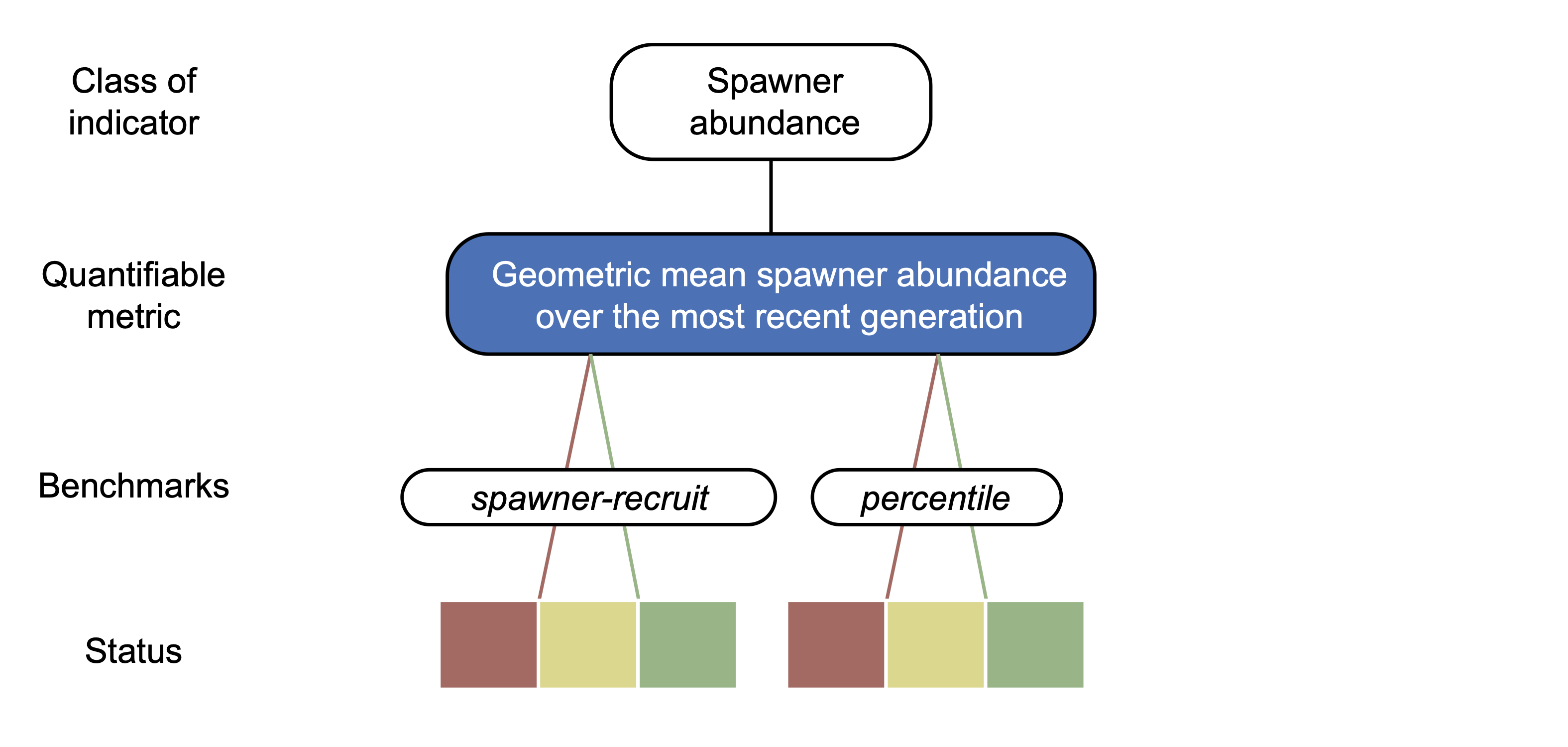
Figure 4.2: Illustration of the Wild Salmon Policy status assessment framework (adapted from Holt et al., 2009). In order to determine the biological status for a given CU, we focus on the geometric mean spawner abundance (metric, blue) under the spawner abundance indicator.

The status of each CU is then assessed by comparing the current spawner abundance, calculated as the geometric mean spawner abundance in the most recent generation, to the upper and lower benchmarks. The number of years in a generation is CU-specific based on information about the life-history of each CU. Where CU-specific data on age-at-return are unavailable, we assume generation lengths of 5 years for Chinook CUs, 4 years for coho CUs, 4 years for chum CUs, and 4 years for sockeye CUs. Pink salmon have a consistent 2-year age-at-return and because even- and odd-year lineages are considered separate CUs, the most recent spawner abundance is simply the most recent year’s estimated spawner abundance for this species. A CU is assigned a red status if the current spawner abundance is at or below the lower benchmark, an amber status if the current spawner abundance is above the lower benchmark and at or below the upper benchmark, and a green status if it is above the upper benchmark.

As spawner-recruit benchmarks consider both productivity and carrying capacity of each CU, they are more biologically meaningful, and we aim to apply them whenever possible. However, spawner-recruit benchmarks require spawner abundance and additional data at the CU-level (e.g. age structure and exploitation rates) that may not be available for a given CU. When these data are not available, we calculate benchmarks based on percentiles of historical spawner abundance, referred to as percentile benchmarks. Percentile benchmarks have been shown to approximate spawner-recruit benchmarks (Holt et al. 2018). Except for specific cases (detailed below), they can be a suitable alternative to spawner-recruit benchmarks when the necessary data to estimate spawner-recruit curves are unavailable.

4.1.4.1 Spawner-Recruit Benchmarks

We use a Ricker model to describe the spawner-recruit relationship and define associated benchmarks:

\[R_{i,t} = S_{i,t} \exp(a_i - b_i S_{i,t}) \] where \(R_{i,t}\) is the number of recruits for CU \(i\) and brood year \(t\), \(S_{i,t}\) is the total number of spawners for CU \(i\) in year \(t\), \(a_i\) is the CU-level intrinsic productivity parameter that describes the population growth at low spawner abundance, and \(b_i\) is the density-dependence parameter.

A target reference point commonly applied in fisheries is the number of spawners that produces maximum sustainable yield, or \(S_{MSY}\), where yield is \(Y = R - S\). This can be calculated from the above Ricker equation given parameters \(a\) and \(b\):

\[ S_{MSY} = \frac{1-W(e^{1-a})}{b}\] where \(W\) is the Lambert W function (Scheuerell 2016). Following recommendations under Canada’s Wild Salmon Policy and to be consistent with DFO’s Decision-Making Framework, we apply an upper spawner-recruit benchmark equal to 80% of \(S_{MSY}\) [Holt et al. (2009). The lower spawner-recruit benchmark \(S_{GEN}\) is the spawner abundance that leads to \(S_{MSY}\) in one generation assuming consistent environmental conditions and no harvest.

To estimate Ricker parameters \(a_i\) and \(b_i\) for each CU \(i\), we apply a hierarchical Bayesian model to spawner-recruit data for all CUs within a species and region combination. The hierarchical model includes hyperparameters for productivity such that data-poor CUs can borrow information from data-rich CUs of the same species within the region to improve parameter estimates. Specifically, each \(a_i\) parameter is drawn from a log-normal hyper distribution: \[a_i \sim \text{Normal} \left( \mu_a, \sigma_a \right) \] where \(\mu_a\) is the mean productivity among all CUs for the given region and species and \(\sigma_a\) is the standard deviation in productivity parameters among CUs for the given region and species.

The density-dependence parameter is estimated independently for each CU using CU-specific prior information: \[ b_i \sim \text{logNormal} \left( \log \left( \frac{1}{S_{\text{max},i}} \right), \sigma_{b,i} \right) \] where \(S_{\text{max},i}\) is the maximum spawner abundance for CU \(i\) and \(\sigma_{b,i}\) is the standard deviation of \(b_i\) for CU \(i\). If habitat capacity data are available and its use is supported by published literature and expert opinion, we use this information to estimate \(S_{\text{max},i}\) as an informative prior on \(b_i\). To date, habitat capacity data has only been available for lake-type sockeye CUs. Estimates of \(\sigma_{b,i}\) represent the degree of certainty in the prior on \(S_{\text{max},i}\): for lake-type sockeye with estimates of habitat capacity we assumed \(\sigma_{b,i} = 0.3\), except for the four Babine system CUs in the Skeena Region where the prior was minimally informative and \(\sigma_{b,i} = 1\) (Korman and English 2013). For other species, we assumed that the mean of the prior for \(S_{\text{max},i}\) was equivalent to the average escapement, and used highly uninformative (\(\sigma_{b,i} = 10\)) or minimally informative (\(\sigma_{b,i} = 1\)) prior distributions following Korman and English (2013).

We estimate parameters \(a_i\) and \(b_i\) for each CU \(i\) by fitting the linearized Ricker model to spawner and recruit data: \[ \log \left( \frac{R_{i,t}}{S_{i,t}} \right) = a_i - b_i S_{i,t}\] where \(a_i\) is drawn from a region/species hyperdistribution as described above, with priors \(\log (\mu_a) \sim N(0.5, 1000)\), \(\sigma_a = \sqrt(1/\tau_a)\) where \(\tau_a \sim \text{Gamma}(0.5, 0.5)\). The above linearized Ricker model is fit to all CUs for a given region and species together using the R package R2jags (Su and Yajima 2021), with a total number of iterations of 100,000, removing 5000 iterations for burnin and applying a thinning interval of 10. The resulting posterior draws for \(a_i\) and \(b_i\) are used to calculate posteriors for \(S_{MSY}\) and \(S_{GEN}\). The posteriors for these upper and lower benchmarks are summarized by calculating the highest posterior density (HPD) and 95% highest posterior density interval (HPDI). We chose to use these summary statistics instead of the mean or median because the posteriors for \(S_{MSY}\) and \(S_{GEN}\) were, in some cases, quite skewed given the tendancy for spawner abundance to be log-normally distributed. For CUs with extremely low productivity, \(S_{MSY}\) can be less than \(S_{GEN}\), yielding benchmark values that do not make biological sense (Holt et al. 2018; Peacock et al. 2020). We do not use spawner-recruit benchmarks in these cases and instead apply percentile benchmarks.

Biological status of each CU is assessed by comparing the geometric mean spawner abundance over the most recent generation against upper and lower benchmarks. We compare the geometric mean spawner abundance against all posterior draws of \(S_{MSY}\) and \(S_{GEN}\) to yield a probability of a CU having each status outcome. The status colour shown on the Pacific Salmon Explorer is the most likely outcome (i.e. the one with the highest posterior probability). The HPD and 95% HPDI for the lower and upper spawner-recruit benchmarks are also shown. See Korman and English (2013) for further details, including a discussion of uncertainty and possible biases in benchmarks and status assessments derived from spawner-recruit models.

4.1.4.2 Percentile Benchmarks

To quantify biological status using percentile benchmarks, we define the lower and upper benchmarks as the 25th (\(S_{25}\)) and 50th (\(S_{50}\)) percentiles of historical spawner abundance, respectively. The upper benchmark (\(S_{50}\)) approximates the upper spawner-recruit benchmark of 80% \(S_{MSY}\) (Holt et al. 2018). We then determine the biological status of each CU by comparing the geometric mean of spawner abundance over the most recent generation to these upper and lower benchmarks. For example, a CU is assessed as red status if the current estimate of spawner abundance is at or below the 25th percentile of historical spawner abundance, amber status if the current average spawner abundance is between the 25th and 50th percentiles of historical spawner abundance, and green status if the current average spawner abundance is at or over the 50th percentile.

We also generate and display 95% confidence intervals around the upper and lower percentile benchmarks using a model-based computational approach that accounts for autocorrelation in the spawner abundance time series. First, we fit a simple autoregressive (AR) model to the time series of log spawner abundances for each CU to estimate the temporal autocorrelation, using the R function ar. We calculate the temporal autocorrelation, \(\phi_1\), for a lag of one year (further consideration may want to be given to including other lags). Next, we extract the residuals from the fitted series and sample from those residuals with replacement to generate \(n\) time series of bootstrapped residuals, each with length equal to the length of the original spawner abundance time series. Finally, we simulate \(n\) new time series using the estimated autocorrelation and bootstrapped residuals. The equation for simulated spawner abundance time series is: \[ \log(S_{i,t}) = \bar{S} + \phi_1 \left( \log (S_{i,t-1}) - \bar{S} \right) + \epsilon_{i,t} \] where \(S_{i,t}\) is the simulated spawner abundance at time \(t\) for the \(i\)th simulation, \(\bar{S}\) is the mean spawner abundance as estimated from the AR model, \(\phi_1\) is the temporal autocorrelation estimated from the AR model, and \(\epsilon_{i,t}\) is the bootstrapped residual for simulation \(i\) and timestep \(t\).

For each of the \(n\) simulated time series, we calculate the 25th and 50th percentiles of spawner abundance. We then take the 2.5th and 97.5th quantiles of the \(n\) estimates of these lower and upper benchmarks to yield bootstrapped 95% confidence intervals on \(S_{25}\) and \(S_{50}\).

4.1.4.3 Additional Status Assessments

In addition to the standardized assessments of biological status developed by the Pacific Salmon Foundation on the Pacific Salmon Explorer, we also display Wild Salmon Policy (WSP) status assessments completed by Fisheries and Oceans Canada (DFO), assessments conducted by the Committee on the Status of Endangered Wildlife in Canada (COSEWIC), and/or assessments conducted by the Province of BC where available (Appendix 3). About 10% of salmon CUs in BC have status assessments completed by DFO for the WSP and/or by COSEWIC (e.g. Committee on the Status of Endangered Wildlife in Canada 2017, 2018; Fisheries and Oceans Canada (DFO) 2018). These assessments apply multiple metrics and expert judgment to assess status and focus primarily on economically significant Chinook, sockeye, and coho CUs in the Fraser and south coast of BC. Fisheries and Oceans Canada does not lead status assessments for steelhead under the WSP, but the Province of BC conducts biological status assessments for some steelhead populations following the Ministry of Forests, Lands, and Natural Resource Operations Fish and Wildlife Branch (2016). For steelhead CUs, we visualize the outcomes of Province of BC status where these assessments are documented and conducted at comparable scales to steelhead CUs. When available, we display the WSP, COSEWIC and Province of BC status assessments alongside the standardized status assessments completed by PSF. In some cases, statuses may differ between the different assessments due to varying approaches to status evaluation and/or different years of data being used.

4.1.4.4 Decision Rules for Assessing Biological Status

Deciding which benchmarks are most appropriate for assessing the biological status of a given CU depends on the available data. With input from the Population Science Advisory Committee, we have developed a set of decision rules to guide how we apply benchmarks to assess biological status for all CUs on the Pacific Salmon Explorer (Figure 4.3).

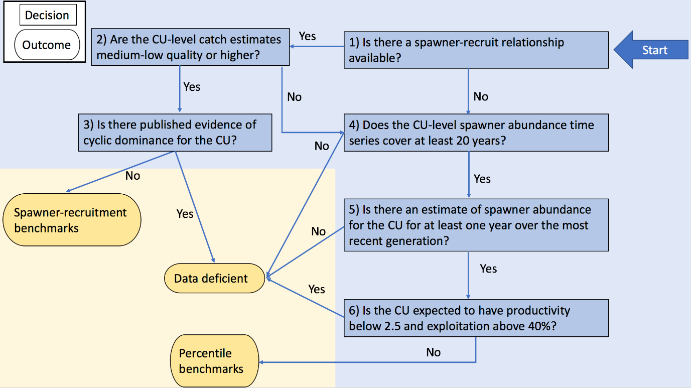
Figure 4.3: Flowchart for documenting decision rules for quantifying biological status.

We use the following guiding questions to determine which benchmarks to apply given the available data for a CU.

1. Is there an estimate of spawner abundance for the CU for at least one year over the most recent generation?

We require at least one annual estimate of spawner abundance over the most recent generation to quantify current spawner abundance. We then take the geometric mean of current spawner abundance over the most recent generation to compare to the estimated benchmarks for that CU to assess biological status.

2. Is there a spawner-recruit relationship available with CU-level catch estimates medium-low quality or higher?

A spawner-recruit relationship must be available to calculate spawner-recruit benchmarks. Most spawner-recruit relationships have over 10 data points (see Appendix 3). Furthermore, errors in estimating catch can lead to misclassification of status using spawner-recruit benchmarks (Peacock et al. 2020). As such, we do not apply spawner-recruit when CU-level catch estimates are highly uncertain (i.e. the data quality score for catch estimates is low; see Data Quality).

3. Is there published evidence of cyclic dominance for the CU?

Some CUs have population dynamics characterized by cyclic dominance (e.g. a four-year generation length that involves a dominant brood year that is most abundant, a sub-dominant brood year, followed by two brood lines with lower abundance). For these cyclic dominant CUs we do not pool data across brood lines to generate estimates of current spawner abundance or to generate CU-level benchmarks because spawner abundance is so different from year to year (Grant et al. 2020). For these CUs, we currently only visualize biological status assessments on the Pacific Salmon Explorer developed through integrated status assessments that incorporate expert judgment and quantitative modeling, where available (e.g. Fisheries and Oceans Canada (DFO) 2018).

4. Does the CU-level spawner abundance time series span at least 20 years?

Estimates of spawner abundance over a relatively long time series are required to assess the biological status of a CU. We require a minimum of 20 years of annual estimates of spawner abundance, although we do not require that these estimates are continuous. In some cases, we may use only a subset of the available time series. We do this if expert opinion suggests that using the entire time series is not appropriate.

5. Is the CU expected to have productivity less than 2.5 and/or exploitation greater than 40% ?

In most circumstances, we do not apply percentile benchmarks if productivity is low (< 2.5) and/or fisheries exploitation is high (> 40%). In these cases, percentile benchmarks can result in biological status assessments that are overly optimistic and, therefore, risky from a long-term management perspective (Holt et al. 2018; Peacock et al. 2020).

6. Is the status outcome in the Red (Poor) category based on percentile benchmarks?

For cases where there is information to suggest that a CU is experiencing productivity below 2.5 and/or exploitation above 40%, we will only report on status outcomes based on percentile benchmarks if the status is in the red zone. In these cases, the potential bias will not have resulted in an overly optimistic status outcome because the red status zone is the lowest status zone.

The spawner-recruit benchmarks modelling approach can sometimes result in lower benchmarks (\(S_{GEN}\)) exceeding upper benchmarks (80% of \(S_{MSY}\)). In such instances, we employ the percentile benchmark approach.

For a number of CUs across all Regions, data limitations mean that we cannot assess the current biological status. In these cases, we categorize these CUs as data deficient. We consider two types of data deficiencies when assessing biological status for the Pacific Salmon Explorer. First, some CUs have no data on spawner abundance for the most recent generation, which prevent us from generating an estimate of current abundance to compare against the benchmarks and assess biological status. Second, in some casses, the time series of spwaner data does not include 20 years of data and we consider the status of these CUs data deficient. There are also two cases where we do not assess the biological status of CUs even though long, current time series may exist (i.e. “not assessed”). First, for CUs that display cyclic dominance, we do not apply either spawner-recruitment or percentile benchmarks. Second, for CUs without spawner-recruit data, that have low productivity and/or high exploitation, and have a green or amber status, we do not assess biological status.

Given the iterative and incremental development approach that we take to visualizing salmon data and assessing biological status, the current set of decision rules outlined in this technical report are subject to change to ensure that our methods align with current best practices for quantifying biological status. As such, the methods and decision rules presented here diverge from previously published PSF technical reports documenting our approach to assessing biological status in specific Regions (Connors et al. 2013; Connors et al. 2018, 2019).

4.1.5 Extinct, De Novo, and Transplant CUs

Over time, DFO may re-classify CUs if: 1) CU-level spawner abundance declines to a point where the CU is lost (“extinct”), 2) a CU is extinct and then re-introduced with different genetic stock (“de novo”), 3) a CU is created by introducing populations to a location where they were not previously present (“transplant”). We visualize these categories on the Pacific Salmon Explorer, intending to maintain a historical record of Pacific salmon’s changing genetic diversity and abundance (see Appendix 1 and Appendix 3).

4.1.6 Limitations: Biological Status Assessments

There are a number of limitations to the biological status assessments that we visualize on the Pacific Salmon Explorer. Some limitations, such as CU-level estimates of spawner abundance, developing benchmarks, and monitoring coverage, apply to all species and Regions. These caveats should be considered when interpreting the results of the biological status assessments and included in future research priorities.

4.1.6.1 CU-level Estimates of Spawner Abundance

If a complete census or true count of spawners is not available for all streams within a CU, DFO applies expansion factors to generate CU-level estimates of spawner abundance. The number of indicator streams that are counted in a given year for each CU (spawner survey coverage) has been declining since the late 1990s in many Regions included in the Pacific Salmon Explorer (e.g. English et al. 2018), leading to increasing uncertainty when extrapolating from spawner counts at monitored streams to CU-level estimates of spawner abundance. This is particularly problematic if the realtive contribution of streams within a CU changes through time. Nonetheless, the expansion factor approach applied by DFO is generally recognized as the best practice for generating CU-level estimates of spawner abundance in many cases [e.g. on the North and Central Coast; English (2012)). Our work aims to derive biological status assessments of individual CUs relative to benchmarks and not, for example, to set management targets or catch allocation, so the assumptions that support these expansion procedures should not overly influence this work.

In addition, recent simulation analyses to determine the influence of these expansion factors on biological status assessments using our approach found that they were robust to a range of expansion procedures (Peacock et al. 2020). Peacock et al. (2020) suggest that, under certain conditions, declining monitoring coverage (to a point) has little impact on the accuracy of benchmarks or biological status assessments using our methods. We have also attempted to account for differing levels of monitoring coverage as part of our work to quantify data quality for visualization on the Pacific Salmon Explorer (see Data Quality).

4.1.6.2 Refining benchmarks

We have developed the benchmarks to assess biological status based on the latest and most comprehensive available literature and in consultation with our Population Science Advisory Committee. However, we recognize the existence of alternative approaches, and we are committed to continuously assess and refine our iterative approach using best practices. For example, if available, habitat-based benchmarks (e.g. Parken et al. 2006) could be applied to situations where other biological benchmarks cannot be used.

4.1.6.3 Other Limitations

Other limitations are species- or Region-specific; the latter are included below in the Regions section.

4.2 Habitat Status: Indicators & Benchmarks

Our assessments of habitat status that we complete and visualize on the Pacific Salmon Explorer follow the approaches developed for evaluating status under Strategy 2 of the Wild Salmon Policy (Fisheries and Oceans Canada 2005). Following this guidance, monitoring should be informed by information on a suite of habitat indicators. Habitat indicators provide a measure of the characteristics of the environment, such as the habitat condition, magnitude of stress, degree of exposure to a stressor, or ecological response to exposure. To evaluate the potential risk of degradation to freshwater salmon habitat, each indicator should be relevant to salmon and represent a clear scientific understanding of either a direct or an indirect relationship between its measurement and its impact on salmon.

Habitat indicators can be further described as either pressure indicators or state indicators following the two-tiered pressure and state indicator framework described by Stalberg et al. (2009). Pressure indicators are natural processes or human activities that can directly or indirectly induce qualitative or quantitative changes in environmental conditions (Stalberg et al. 2009). State indicators are physical, chemical, or biological attributes measured to characterize environmental conditions on the ground (Stalberg et al. 2009). Distinguishing features between pressure and state indicators include the scale of assessment, the resolution of input data, and the cost of assessment and monitoring. Pressure indicators are often assessed for large geographic areas using remotely sensed information. Evaluation and quantification of pressure indicators are generally less resource intensive than for state indicators because the associated data collection does not typically require on-the-ground field studies. State indicators on the other hand are typically assessed over smaller geographic areas than for pressure indicators, often requiring higher resolution data to evaluate and quantify, and require more resources as they often depend on associated on-the-ground fieldwork. Our work to date has focused on evaluating pressure indicators as the first step to gaining an understanding of habitat conditions over broad regional and provincial-scale geographic extents. Assessments of habitat pressure indicators across the province is intended to help identify priority areas to conduct finer-scale assessments of key habitat state indicators.

Through engagement with an expert Habitat Science Advisory Group (HSAC) we have identified a set of seven “core” pressure indicators affecting salmon habitats that are to be assessed and visualized within the Pacific Salmon Explorer. These selected core habitat pressure indicators include: forest harvest, fire, insect damage, roads, urban and industrial development, agriculture, and mines. The intent of these core pressure indicators is that in composite they represent the primary suite of broad-scale land disturbances directing or indirectly impacting freshwater habitats. For each of these core pressure indicators we have defined defensible literature-defined empirically-based “threat” benchmark values that can be applied across provincial watersheds for ascribing the relative level of concern (i.e., low, medium, high) in regards to their potential degradation of salmon habitats.

4.2.1 Scale of Habitat Assessments

The base reporting unit for our assessments of habitat pressure indicators are the 1:20,000 Freshwater Atlas (FWA) assessment watersheds dataset (BC Ministry of Environment (MOE) 2017a). A map of all the FWA watersheds in BC is available in Appendix 4. The Freshwater Atlas is the most comprehensive, standardized source of hydrologic features in BC. FWA assessment watersheds are a commonly used provincial baseline dataset for resource managers, researchers, and others interested in evaluating and reporting at a watershed scale. The FWA assessment watersheds replace the legacy 1:50,000 BC Watershed Atlas Third-Order Watersheds dataset. FWA assessment watersheds are delineated at a scale where hillslope and channel processes are generally well linked, between 2,000 to 10,000 hectares (Carver and Gray 2009).

4.2.2 Mapping Salmon Spawning Locations

We need to know where salmon spawn and rear to identify where habitat pressures could be most affecting salmon. We use observations of spawning and rearing locations to identify and delineate local salmon habitats, delineate the extent of upland areas that may also impact these habitats through downstream processes, and use this information to determine the relevant spatial extent for habitat assessments. We identify salmon spawning locations using several key data sources: The Fisheries Information Summary System (FISS) database, technical reports, maps, additional databases when available, and local knowledge derived through expert elicitation. We also identify rearing locations through the same sources. However, specific salmon rearing locations are generally not as well-known as for spawning and so direct observations of rearing may be supplemented by modelled information on predicted extent of rearing distribution.

4.2.2.1 Fisheries Information Summary System

The FISS database is a legacy project which was a jointly funded initiative between BC Fisheries and DFO, intending to provide fish habitat data for water bodies throughout BC and the Yukon (BC Ministry of Environment (MOE) 2017b). FISS data is distributed under two datasets via DataBC on the BC Data Catalogue. The two datasets, specifically, are BC Historical Fish Distribution Zones (50,000) and Known BC Fish Observations and BC Fish Distributions. The latter dataset is described as “the most current and comprehensive information source on fish presence for the province” on DataBC.

As of 2001, the Province of BC no longer maintains the spawning zones or linear distribution dataset (“BC Historical Fish Distribution - Zones (50,000)”), but the Known BC Fish Observations and BC Fish Distributions dataset is actively maintained. This dataset houses the legacy FISS data as well as data from other provincially maintained sources. However, efforts to maintain fish location data are not standardized province-wide, and thus both data coverage and accuracy vary across BC. The province continues to document ongoing data submissions from organizations or individuals required to report fisheries data and sampling information as part of the reporting requirements for a Scientific Fish Collection Permit (a permit to capture or collect fish specimens for scientific or other non-recreational or commercial purposes). The province also documents submissions of non-permitted fish and fish habitat information on a voluntary basis. While presenting some challenges, these datasets are the most comprehensive source of spawning data available province-wide, so we use them as a base representation of spawning locations. We filtered these datasets to Pacific salmon species and spawning activity types to identify spawning locations.

4.2.2.2 Additional Technical Reports, Maps, and Databases

In some Regions, we have worked with technical committees and local salmon experts to identify additional spawning or habitat information available within technical reports, previously published maps, and other databases (see Regions).

4.2.2.3 Expert-elicited Spawning Location Information and Data Review

Given the limitations of the provincially available datasets, we work with local expert knowledge holders in each of our Regions to review and supplement the existing spawning location information using hard copy paper maps and our ESRI-based mapping platform, the salmon Habitat Mapper (Figure 4.4). We use a structured process whereby we 1) compile large-format paper maps of each study area that include spawning location data, and 2) use the salmon Habitat Mapper, a private online tool that we developed for exploring and contributing spawning data. Using these two tools, we work with project partners who have local knowledge of where salmon spawn in each Region to review and update spawning location data. These review sessions typically include both fisheries staff and community members who work with us over a day-long workshop in their local area within a Region. Any additional data documented via the large-format paper maps are then digitized and integrated, along with data collected via the salmon Habitat Mapper, into our spawning locations dataset.

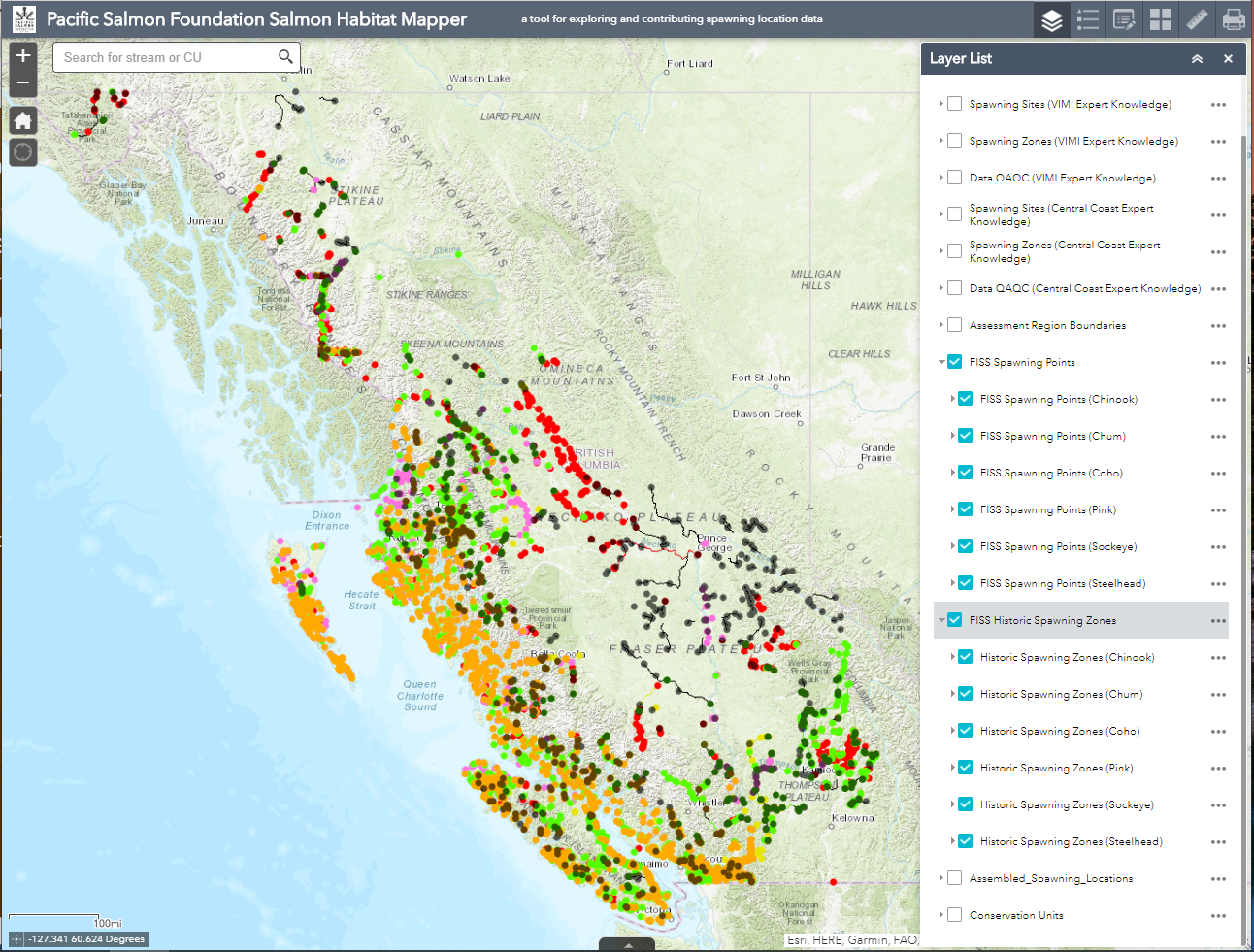
Figure 4.4: salmon Habitat Mapper: A Collaborative Tool for Mapping salmon Spawning Habitats.

4.2.2.4 Assigning Spawning Locations to Conservation Units

For all spawning location information, we assign observed locations to individual CUs. For all species except lake-type sockeye, we assign spawning locations to CUs by determining CU overlap with spawning site locations. This is done on a species-specific basis, except for pink CUs. If spawning location data sources did not differentiate between even-year or odd-year pink, we attribute that spawning location to both even-year and odd-year pink CUs in that area (where applicable). For lake-type sockeye, CU boundaries tend to be constrained to a rearing lake, so to capture the side channels where salmon spawn, we use the defined rearing lake zone of influence to locate associated spawning sites. Any sockeye spawning locations that are situated outside our defined lake-type sockeye spawning zones of influence are instead considered to be associated with an overlapping river-type Sockeye CU and are assigned accordingly.

4.2.3 Identifying Salmon Spawning Habitat

Our assessment methodology uses the concept of a zone of influence (ZOI) to identify the extent of land considered to influence particular freshwater salmon habitat, including areas upstream. Using ZOIs to assess salmon freshwater habitats aligns with Strategy 2 of the Wild Salmon Policy, in that 1) the identification of habitats that support or limit salmon production is necessary to inform assessment, monitoring, and protection priorities; and 2) that habitat requirements vary by species, life history characteristics and phase, and geography (Fisheries and Oceans Canada 2005).

• We define ZOIs for the for each salmon CU. A ZOI represents the area of land that drains into the spawning and/or rearing habitats used by a specific salmon CU.

We use the geographic extents of ZOIs to assess and quantify habitat pressures by CUs for both the spawning and rearing life stages. The specific rules for defining ZOIs were originally developed in collaboration with PSF’s Skeena Technical Advisory Committee (Porter et al. 2013, 2014) and are defined in Appendix 5 with species and Region-specific nuances, where relevant.

4.2.4 Overview of Habitat Pressure Indicators

Once we have identified salmon habitat and ZOIs, we use a set of habitat pressure indicators to derive coarse-scale assessments of pressures on salmon freshwater habitats. We developed a set of habitat pressure indicators during our initial methodology development with the Skeena Technical Advisory Committee (Porter et al. 2013, 2014) that built off the recommendations for monitoring and evaluation of salmon habitats under the Wild Salmon Policy (Stalberg et al. 2009). We have continued to refine our indicator through ongoing consultation with our Habitat Science Advisory Committee that has identified this reduced “core” set of habitat pressure indicators that we can evaluate consistently across all watersheds in the province. The seven core indicators are: 1. Forest Harvest 2. Fire 3. Insect Damage 4. Roads 5. Urban & Industrial Development 6. Agriculture 7. Mines

Descriptions of each of these indicators are provided in Table 4.13.

Table 4.13: Habitat pressure indicator definitions and their relevance to salmon habitat. (Note that watershed refers to the Province of British Columbia’s 1:20,000 Freshwater Atlas (FWA) Assessment Watersheds.)

Indicator	Definition	Relevance	Pressure Metric
Forest Harvest	Areas within a watershed where trees have been cut and removed for processing at sawmills or pulp mills.	Forest harvest (logging) results in a reduction in forest cover that can change watershed hydrology by affecting rainfall interception, transpiration, and snowmelt processes. Such changes in hydrology can affect salmon habitats through altered peak flows, low flows, annual water yields, and elevated stream temperatures.	% of total watershed area that has been harvested in the last 60 years (with disturbance effects adjusted by time since forest harvest).
Fire	Areas within a watershed where there has been combustion of forests and woodlands.	Fires can result in a reduction in forest cover that can change watershed hydrology by affecting rainfall interception, transpiration, and snowmelt processes. Such changes in hydrology can affect salmon habitats through altered peak flows, low flows, annual water yields, and elevated stream temperatures.	% of total watershed area that has burned in the last 60 years (with disturbance effects adjusted by both time since burn disturbance and severity of burn).
Insect Damage	Areas within a watershed that have experienced intense and prolonged attacks of native or non-native xylophagous (e.g. bark beetles) or folivorous (e.g. defoliators) insect pests that have caused extensive tree mortality.	Damage to and death of trees due to insect attacks can result in a reduction in forest cover that can change watershed hydrology by affecting rainfall interception, transpiration, and snowmelt processes. Such changes in hydrology can affect salmon habitats through altered peak flows, low flows, and annual water yields.	% of total watershed area damaged by insect pests in the last 60 years (with disturbance effects adjusted by both time since pest disturbance and severity of pest-induced forest mortality).
Roads	Linear corridors within a watershed that have been cleared of vegetation and engineered to allow travel by motorized vehicles on paved, gravel, or dirt surfaces.	Road development can interrupt subsurface flow, increase peak flows, and interfere with natural patterns of overland water flow in a watershed. Roads can be a significant cause of increased erosion and fine sediment deposition in streams, which can impact salmon spawning and rearing habitats.	km/km2 density of roads, measured as total road length divided by total watershed area.
Urban & Industrial Development	Areas within a watershed that have been converted from natural landscapes to support urban or industrial development.	Urban and/or industrial land uses expand the area of impenetrable land surfaces (e.g., roads, parking lots, sidewalks), which can substantially increase watershed runoff. This can upset the dynamic equilibrium between the watershed and stream channel, resulting in dramatic changes in stream morphology, increased bank erosion, and overall habitat degradation. Urban land use also directly reduces stream water quality by delivering toxic materials and nutrients to the stream during storms.	% of total watershed area with urban or industrial development.
Agriculture	Areas within a watershed that have been converted from natural landscapes to support agricultural production (i.e. crops or livestock).	Agricultural development can increase runoff in a watershed, destabilizing flows, water temperatures, and channel morphologies in stream habitats used by salmon. Agriculture can also impact water and habitat quality through the introduction of contaminants and nutrients found in agricultural herbicides and fertilizers, and a reduced supply of coarse organic matter for spawning and rearing.	% of total watershed area with agricultural development.
Mines	Locations within a watershed that have been excavated for removal of coal, minerals, or gravel.	The footprint of a mine and mining activity can change geomorphology and the hydrological processes of nearby water bodies. Runoff from mines can also introduce fine sediments and toxic contaminants into streams, impairing water quality, salmon prey densities, and overall survival and productivity of salmon.	#/km2 density of mining, measured as the total number of coal and metal mines, divided by total watershed area.

4.2.4.1 Data Sources

We use specific inclusion criteria to select the datasets we use to inform these habitat pressure indicators to ensure that our methodologies are standardized across Regions. The data that we include must be:

• Publicly available and readily accessible;
• Created with consistent and documented data collection protocols;
• Formatted to allow easy integration into our existing data systems;
• Cost-effective for long-term data collection;
• Reflective of both short- and long-term responses and trends in a given indicator;
• Appropriate to the geographic scale of analysis;
• Supported by quality assurance/quality control protocols and an established data update process.

The data we use to inform the seven core habitat pressure indicators are sourced from publicly available provincial or federal agency databases. The publication year for indicator datasets is between 1992 and 2023 (see Appendix 6 for a complete listing of datasets, publication years, and data sources).

4.2.4.2 Data Processing

We quantify each indicator at the scale of the 1:20,000 FWA assessment watersheds using ArcGIS Pro and a python-scripted ArcGIS Model Builder toolbox. Data processing generally follows a process of selecting features of interest from each indicator dataset and intersecting those with FWA watersheds to quantify habitat pressures by watershed (see Appendix 7 for a complete description of processing methods for each indicator).

4.2.5 Approach to Assessing Cumulative Habitat Pressures

Distinct landscape pressures in a watershed can both an individual impact on the condition of salmon habitats and can also interact and combine with other pressures for even greater potential cumulative impact. We develop cumulative pressure scores for each FWA assessment watershed across CUs and Regions in the Pacific Salmon Explorer to reflect these interactions and better represent that concerns for habitat degradation posed by cumulative pressures. This approach allows us to visualize which CUs face the greatest potential cumulative threat to habitat conditions based on the set of pressure indicators that we assess. Cumulative scores are useful for providing a baseline to consider future threats and identify priority areas to avoid further impacts. A cumulative pressure score also provides a summary index to consider pressures on salmon habitat in relation to the biological status of CUs. This information can help in prioritizing conservation efforts, mitigation strategies, and identifying areas for monitoring state indicators at a higher resolution.

Aggregating indicators into a single, composite threat or condition score is an approach taken by a variety of programs that currently monitor watersheds in Canada and the U.S. Pacific Northwest (e.g. FLNRORD’s Forest and Range Evaluation Program, USEPA’s Environmental Monitoring and Assessment Program, USDA Forest Service’s Aquatic and Riparian Effectiveness Monitoring Program). These programs use a variety of methods to aggregate their habitat data, and each approach has strengths and weaknesses (Pickard et al. 2008). Habitat indicator analyses for BC salmon CUs [e.g. Cohen Commission analyses of Fraser sockeye CUs; Nelitz et al. (2011)] and an indicator-mapping project for the Lower Thompson coho CU (Beauchamp 2008) generated cumulative habitat stressor or impact scores based on a simple summation of all the individually scored indicators (i.e. a higher total score equates to higher threat). Habitat assessments for southern BC Chinook CUs (Porter et al. 2013) employed an alternative approach for rating relative risk in watersheds whereby cumulative risk scoring was based on an indicator ‘roll-up’ rule set based on the proportion of the indicators that were rated low, moderate, or high threat.

For the habitat pressure assessments included in the Pacific Salmon Explorer, we apply a set of roll-up rules to assign cumulative pressure scores. We calculate this cumulative pressure score for individual 1:20,000 FWA assessment watersheds within the zones of influence of all CUs. Any Region-specific idiosyncrasies are documented within the Regions section.

4.2.6 Limitations: Habitat Pressure Indicators & Analysis Methods

While the current suite of habitat pressure indicators has been developed according to Wild Salmon Policy guidelines (Stalberg et al. 2009), they do not reflect all of the pressures on wild salmon. Understanding the full range of pressures on salmon requires additionally documenting marine habitat pressures, climate change indicators, and developing a deeper understanding of fisheries pressure, to name a few. Given the set of habitat pressure indicators that we currently include on the Pacific Salmon Explorer, specific limitations of our approach relate to outdated and incomplete datasets, benchmark uncertainty, and methods for calculating cumulative pressure scores. These limitations apply to all Regions, species, and CUs that we include in the Pacific Salmon Explorer and should be considered as both caveats to the current habitat assessment results as well as future research priorities.

4.2.6.1 Data Needs

Incomplete and outdated datasets are a continued challenge for completing coarse-scale assessments of threats to freshwater habitats. For example, information on land cover classifications was dated between 1996-2005 and the Baseline Thematic Mapping dataset was produced in the 1990s. These are examples where more current datasets certainly exist but are either not yet publicly available or may not be available at broad spatial scales.

Overall, temporal and spatial data gaps limit our ability to quantify and assess current freshwater salmon habitat threats accurately. Better and more current spatial data are needed to support a more accurate and up-to-date assessment of pressures on freshwater salmon habitats across all Regions.

4.2.6.2 Refining Benchmarks

Additional research is needed to refine the science-based benchmarks we are using for our core habitat pressure indicators and to develop such benchmarks for other habitat pressures.

4.2.6.3 Cumulative Pressure Scores

The approach we use to calculate overall cumulative pressure scores for freshwater salmon habitats is a roll-up rule set. This approach assumes that each indicator is weighted equally in terms of the overall cumulative pressure score. We do not weight certain indicators as having more or less impact on salmon habitat over others. Determining how best to aggregate indicators to calculate overall cumulative pressure scores is a challenge, and while the approach we have used is defensible, transparent, and easily understood by a range of audiences, it is certainly not the only way to aggregate indicators, nor necessarily the best way.

4.2.7 Overview of Habitat State Indicators

Habitat state indicators are defined within Strategy 2 of the WSP (Stalberg et al. 2009) as physical or chemical attributes measured to characterize the environmental conditions within salmon habitats. At a local scale (i.e., watershed or individual CU), habitat managers would be expected to use both pressure and state indicators as available to evaluate habitat status and better understand salmon habitat conservation or restoration priorities. As identified in Stalberg et al. (2009) a requirement for field measurement means that state indicators are generally more difficult and more expensive to monitor than are pressure indicators. Second, high natural variability in habitat conditions may require a high sampling effort to reliably detect meaningful differences or changes in values for habitat state indicators (i.e., low statistical power). Thus, localized monitoring of different habitat state indicators, while of critical importance for understanding the actual on-the-ground condition of salmon habitats, must be designed, analyzed, and interpreted appropriately to allow for integration of such information to inform broader inferences of habitat status across watersheds, CUs, or provincial regions.

Work to quantify habitat state indicators has started with two indicators related to climate changes in salmon watersheds: stream temperature and stream flows.

4.2.7.1 Stream Temperature

Stream temperature is an important variable that structures aquatic ecosystems, dictating the species that can survive and thrive in an area and affecting the behaviour and life-history timing of those present (Ficklin et al. 2023). Stream temperature is generally projected to increase throughout BC and the Yukon with climate change, as air temperatures rise, and hydrologic regimes shift from snow- or glacier-dominated to rainfall-dominated. For example, summer water temperatures in the Fraser River have warmed by ~1.5 °C since the 1950s (British Columbia Ministry of Environment 2015). These rising temperatures may have negative impacts on all freshwater life stages of salmon. We were interested in identifying an indicator that would provide information on increases to stream temperatures that may negatively affect salmonids. We chose to focus on the 7-day running average of the daily maximum temperature (7DADM), which is sensitive to changes in high stream temperatures that persist for a period of several days or more.

To quantify the 7DADM, continuous logger data recorded at hourly intervals are needed because spot measurements may not capture daily maximum temperatures. Although continuous stream temperature monitoring is becoming more prevalent, these data are not compiled and made available by a single agency, such as the Water Survey of Canada does for flow data. We compiled stream temperature data from a variety of sources (4.14) and calculated daily maximum temperatures from the full time series and then calculated the 7DADM. We then performed a basic quality-assurance/quality-control (QA/QC) of the daily maxima through the following steps:

1. Removing values < 0 ˚C
2. Removing values > 30 ˚C
3. Removing values that showed an increase or decrease of more than 2.5 ˚C from the previous day (more than 99% of day-to-day changes were less than +/- 2.3 ˚C)

From the remaining data, we calculated the 7DADM for each location by taking the average of the daily maximum temperatures for the current and previous 6 days (i.e., right-aligned 7-day moving average), ignoring missing data.

In the Pacific Salmon Explorer, stream temperature monitoring locations can be sorted by the station name or by the maximum 7DADM in the most recent year. In the stream temperature overlays, we visualize the median (blue line) and range (grey) of the 7DADM for each day-of-year across all years on record. We also show the daily 7DADM for the most recent year of data. To facilitate the interpretation of these data in the context of what it means for salmon, we show a general 18 ˚C threshold as a horizontal red dashed line.

Table 4.14: Sources of stream temperature data shown in the Pacific Salmon Explorer.

Source	Number of monitoring locations	Median days of data per station (2.5th, 97.5th quantiles)	Date range
Province of BC	266	477 (60, 3050)	1995-2021
Water Survey of Canada	179	1599 (74, 6646)	1996-2022
Yukon River Panel (Al von Finster)	20	1719 (242, 3388)	2011-2020

4.2.7.2 Stream Flow

Climate change is impacting the hydrology of freshwater ecosystems by altering precipitation patterns, reducing the snowpack and hastening glacial retreat, and changing the timing of spring snow melt, leading to more variable flows and changing the timing of peak flows (Ul Islam et al. 2019). The impacts of changing hydrographs on salmon will depend on season and life-stage. However, in general we expect salmon to experience lower flows in late summer and early fall during critical adult migration and spawning periods.

To track when and where critical low flows are occurring, we calculated a 7-day running average of daily flows from the Water Survey of Canada’s HYDAT data for stations in BC and the Yukon. The minimum value for the smoothed flow in each year was compared to the Mean Annual Discharge (MAD) to calculate the minimum % MAD. HYDAT data were downloaded via the tidyhydat R package (Albers 2017), and smoothed daily flows and MAD were calculated for each station using functions in the fasstr R package (Goetz and Schwarz 2022).

For low stream flow, benchmarks for the minimum % MAD follow guidelines from the Province of British Columbia’s Environmental Flow Needs (EFNs) Policy (BC Ministry of Forests, Lands 2022). Specifically, BC’s EFN Risk Assessment Framework assumes that mean monthly discharge: * Greater than 20% lt MAD (long-term mean annual discharge) represent low flow sensitivity; * Between 10 and 20% lt MAD represent moderate flow sensitivity; and * Less than 10% of lt MAD represent high flow sensitivity.

Following this Framework, we visualize a lower benchmark on minimum % MAD of 10% and upper benchmark of 20% when we show annual hydrographs in the Pacific Salmon Explorer.

4.2.8 Limitations: Habitat State Indicators & Analysis Methods

Although the importance of stream temperature to aquatic ecosystems is undisputed, there is no central agency tasked with monitoring and reporting onstream temperature, like the Water Survey of Canada does for river flow and levels. Thus, there are major limitations in both the spatial and temporal coverage of stream temperature data. In particular, there are relatively few time series than span multiple years, making it difficult to identify trends over time. PSF is working to address the general lack of centralized, accessible stream temperature data by working with partners throughout BC and the Yukon to coordinate stream temperature monitoring and compile data into a centralized, quality-controlled database. However, this initiative is in its infancy, and our current stream temperature database may not provide a complete picture of the temperature stress that Pacific salmon may be experiencing throughout their range.

Even where there are stream temperature data, the analysis and interpretation can be challenged by poor data quality or poorly located stations that do not accurately capture conditions experienced by fish. Stream temperature loggers can be displaced or dewatered, resulting in misleading time series. Although we performed an initial QA/QC to remove errors and extreme outliers, due to the large number of stations it is not feasible to examine each time series in detail. Future work could use more sophisticated algorithms and comparison to nearby recorded air temperatures to identify potential dewatering events (e.g., Chezik 2019). We also recognize that rivers are 3-dimensional environments, and there may be considerable fine-scale variability in stream temperature (e.g., thermal refugia) that is not captured by data loggers at a single point location. PSF is working with academics and communities to better understand the thermal landscape of rivers and how this may affect interpretation of stream temperature logger data.

Benchmarks for stream temperature that are specific to salmonids have been identified in BC (Oliver and Fidler 2001) and the US Pacific Northwest (United States Environmental Protection Agency 2003), but new research is uncovering just how variable thermal tolerance can be among salmon populations (Zillig et al. 2021). We have developed the stream-temperature visualizations in a way that is flexible to incorporate different thermal tolerance and optimal temperature ranges for different life-stages, species, and CUs, and will endeavor to update this information to reflect the latest state of knowledge. In the meantime, we recognize that the benchmarks presented may not represent the specific thermal requirements of individuals CUs, and should be used as approximate guidelines. For low stream flow, we assumed a lower benchmark on minimum % MAD of 10% and upper benchmark of 20%. We recognize that many small streams have historically gone dry in the summer months, and that these benchmarks may be overly conservative in these cases where salmon have adapted to low-flow conditions. In other places, flow needs for specific stages and species may be much greater than 20% MAD (Warkentin et al. 2022). Thus, we caution that these are general benchmarks and local considerations must be taken into account when making management decisions.

4.3 Reporting Status Across Spatial Scales

In addition to providing biological and habitat information for individual salmon CUs, we also provide information on the status and trends of salmon populations and their habitats at the Stock Management Unit (SMU) to improve understanding of the current state of salmon at a scale that is highly relevant to fisheries management under the new Fisheries Act. Conservation Units can be grouped and sorted by Stock Management Unit (SMU), based on the provisional list provided by DFO. We are also currently working with DFO to incorporate SMUs into the Pacific Salmon Explorer in additional ways.

Coarser scale assessments of the state of salmon are available through PSF’s companion report: The State of Salmon. This report provides regional summaries of aggregate salmon abundance by species, and highlights key factors affecting Pacific salmon in Canada. While finer-scale data such as CUs are important for supporting the implementation of Canada’s Wild Salmon Policy, coarser-scale synoptic overviews of salmon population status and trends across species and regions are also important for salmon conservation and management. These multi-scale overviews help to improve understanding of patterns in trends and status of salmon CUs across or within Regions and offer insights into potential habitat pressures that could be driving changes in salmon populations. They can also inform regional, provincial, and federal planning and decision-making.

References

Albers, S. 2017. tidyhydat: Extract and Tidy Canadian Hydrometric Data. The Journal of Open Source Software 2(20): 511. doi:10.21105/joss.00511.

BC Ministry of Environment (MOE). 2017a. Freshwater Atlas – Province of British Columbia. Available from https://www2.gov.bc.ca/gov/content/data/geographic-data-services/topographic-data/freshwater.

BC Ministry of Environment (MOE). 2017b. Fisheries information summary system (FISS). Available from https://cmnmaps.ca/DFO_FISS/.

BC Ministry of Forests, Lands, N.R.O. and R.D. 2022. Environmental Flow Needs Policy. Province of British Columbia, Victoria, BC. Available from https://www2.gov.bc.ca/gov/content/environment/air-land-water/water/water-licensing-rights/water-policies/environmental-flow-needs.

Beauchamp, W. 2008. Lower Thompson Coho Conservation Unit indicators mapping project. Prepared for Fisheries and Oceans Canada. Oceans, Habitat and Enhancement Branch (OHEB).

British Columbia Ministry of Environment. 2015. Indicators of Climate Change for British Columbia: 2016 Update. In BC Ministry of Environment and Climate Change Strategy, National Library of Canada.

Brown, G.S., Baillie, S.J., Thiess, M.E., Bailey, R.E., Candy, J.R., Parken, C.K., and Willis, D.M. 2019. Pre-COSEWIC review of southern British Columbia Chinook Salmon (Oncorhynchus tshawytscha) conservation units, Part I: Background. Canadian Science Advisory Secretariat Research Document 2019/011. Available from http://www.dfo-mpo.gc.ca/csas-sccs/.

Brown, G.S., Thiess, M.E., Wor, C., Holt, C.A., Patten, B., Bailey, R.E., Parken, C.K., Baillie, S.J., Candy, J.R., Willis, D.M., Hertz, E., Connors, B., and Pestal, G.P. 2020. 2020 Summary of Abundance Data for Chinook Salmon (Oncorhynchus tshawytscha) in Southern British Columbia, Canada. Canadian Technical Report of Fisheries and Aquatic Sciences 3401: xii + 214 p. Available from https://salmonwatersheds.ca/library/lib_460/.

Carver, M., and Gray, M. 2009. Assessment Watersheds for Regional Level Applications.

Chezik, K.A. 2019. River network structuring of climate and landscape effects in salmon watersheds. Simon Fraser University. Available from https://summit.sfu.ca/item/18782.

Committee on the Status of Endangered Wildlife in Canada. 2017. COSEWIC Assessment and status report on the Chinook Salmon (Oncorhynchus tshawytscha), Okanagan population in Canada. Committee on the Status of Endangered Wildlife in Canada, Ottawa, Canada. Available from https://salmonwatersheds.ca/document/lib_503/.

Committee on the Status of Endangered Wildlife in Canada. 2018. COSEWIC assessment and status report on the Chinook Salmon Oncorhynchus tshawytscha, Designatable Units in Southern British Columbia (Part One – Designatable Units with no or low levels of artificial releases in the last 12 years). Committee on the Status of Endangered Wildlife in Canada, Ottawa, Canada.

Connors, B., Malick, M.J., Ruggerone, G.T., Rand, P., Adkison, M., Irvine, J.R., Campbell, R., and Gorman, K. 2020. Climate and competition influence sockeye salmon population dynamics across the Northeast Pacific Ocean. Canadian Journal of Fisheries and Aquatic Sciences 77(6): 943–949. Available from https://doi.org/10.1139/cjfas-2019-0422.

Connors, B.M., Pickard, D.C., Porter, M., Farrell, G., Bryan, K., Casely, S., and Huang, S. 2013. Skeena Salmon Conservation Unit Snapshots. Report prepared by ESSA Technologies Ltd. for the Pacific Salmon Foundation. Available from https://salmonwatersheds.ca/document/lib_420/.

Connors, K., Hertz, E., Jones, E., Honka, L., Kellock, K., and Alexander, R. 2019. The Nass Region: Snapshots of salmon population status. The Pacific Salmon Foundation, Vancouver, BC. Available from https://salmonwatersheds.ca/library/lib_453/.

Connors, K., Jones, E., Kellock, K., Hertz, E., Honka, L., and Belzile, J. 2018. BC Central Coast: A snapshot of salmon populations and their habitats. The Pacific Salmon Foundation, Vancouver, BC. Available from https://salmonwatersheds.ca/library/lib_442/.

D’Eon-Eggertson, F., Dulvy, N.K., and Peterman, R.M. 2015. Reliable Identification of Declining Populations in an Uncertain World. Conservation Letters 8(2): 86–96. doi:10.1111/conl.12123.

English, K.K. 2012. Extend the time series of catch and escapement estimates for Skeena sockeye, pink, chum, and coho salmon stocks. Available from https://salmonwatersheds.ca/library/lib_262/.

English, K.K. 2016. Review of Escapement Indicator Streams for the North and Central Coast Salmon Monitoring Program Final Report.

English, K.K., Peacock, D., Challenger, W., Noble, C., Beveridge, I., Robichaud, D., Beach, K., Hertz, E., and Connors, K. 2018. North and Central Coast Salmon Escapement, Catch, Run Size and Exploitation Rate Estimates for each Salmon Conservation Unit for 1954-2017. Prepared by LGL Ltd. for the Pacific Salmon Foundation. 125p. Available from https://salmonwatersheds.ca/document/lib_451/.

Ficklin, D.L., Hannah, D.M., Wanders, N., Dugdale, S.J., England, J., Klaus, J., Kelleher, C., Khamis, K., and Charlton, M.B. 2023. Rethinking river water temperature in a changing , human-dominated world. Nature Water 1(February): 125–128. Springer US. doi:10.1038/s44221-023-00027-2.

Fisheries and Oceans Canada. 2005. Canada’s Policy for Conservation of Wild Pacific Salmon. Fisheries and Oceans Canada, Vancouver, BC. Available from https://salmonwatersheds.ca/document/lib_578/ [accessed 23 March 2022].

Fisheries and Oceans Canada (DFO). 2018. The 2017 Fraser sockeye salmon (Oncorhynchus nerka) integrated biological status re-assessment under the Wild Salmon Policy. Canadian Science Advisory Secretariat Research Document 2018/017., Vancouver, BC.

Goetz, J., and Schwarz, C.J. 2022. fasstr: Analyze, Summarize, and Visualize Daily Streamflow Data. Available from https://cran.r-project.org/package=fasstr.

Grant, S.C.H., Holt, C.A., Pestal, G., Davis, B.M., and MacDonald, B.L. 2020. The 2017 Fraser sockeye salmon (Oncorhynchus nerka) integrated biological status re-assessment under the Wild Salmon Policy using standardized metrics and expert judgment. Canadian Science Advisory Secretariat Research Document 2020/038: vii + 211 p. Available from https://waves-vagues.dfo-mpo.gc.ca/library-bibliotheque/40924646.pdf.

Holt, C.A., Cass, A., Holtby, B., and Riddell, B. 2009. Indicators of status and benchmarks for Conservation Units in Canada’s Wild Salmon Policy. Canadian Science Advisory Secreteriat Research Document 2009/058: vii + 74 p. Available from http://www.dfo-mpo.gc.ca/csas-sccs/publications/resdocs-docrech/2009/2009_058-eng.htm.

Holt, C., Davis, B., Dobson, D., Godbout, L., Luedke, W., Tadey, J., and Van Will, P. 2018. Evaluating Benchmarks of Biological Status for Data-limited Populations (Conservation Units) of Pacific Salmon, Focusing on Chum Salmon in Southern BC. DFO Can. Sci. Advis. Sec. Res. Doc. (/011): ix + 87. Available from https://salmonwatersheds.ca/document/lib_580/.

James, S.E., Doherty, B., Cox, S.P., Pearsall, I.A., and Riddell, B. 2023. Size and timing of hatchery releases influence juvenile-to-adult survival rates of British Columbia Chinook (Oncorhynchus tshawytscha) and coho (Oncorhynchus kisutch) salmon. Canadian Journal of Fisheries and Aquatic Sciences 00: 1–19. doi:10.1139/cjfas-2022-0121.

Korman, J., and English, K. 2013. Benchmark Analysis for Pacific Salmon Conservation Units in the Skeena Watershed. Prepared by Ecometric Research Inc. and LGL Ltd. for the Pacific Salmon Foundation, Vancouver, BC. Available from ttps://salmonwatersheds.ca/library/lib_318/.

McMillan, J.R., Morrison, B., Chambers, N., Ruggerone, G., Bernatchez, L., Stanford, J., and Neville, H. 2023. A global synthesis of peer-reviewed research on the effects of hatchery salmonids on wild salmonids. Fisheries Management and Ecology 30: 446–463. doi:10.1111/fme.12643.

Ministry of Forests, Lands, and Natural Resource Operations Fish and Wildlife Branch. 2016. Provincial Framework for Steelhead Management in British Columbia. Available from https://salmonwatersheds.ca/document/lib_560/.

Nelitz, M., Porter, M., Parkinson, K., Wieckowski, K., Marmorek, D., Bryan, K., Hall, A., and Abraham, D. 2011. Evaluating the status of Fraser River sockeye salmon and role of freshwater ecology in their decline. ESSA Technologies Ltd. Cohen Commission Technical Report, 3. Available from https://www.researchgate.net/publication/274721543_Evaluating_the_status_of_Fraser_River_sockeye_salmon_and_role_of_freshwater_ecology_in_their_decline.

Nelitz, M., Wieckowski, K., Porter, M., and Perrin, C. 2007. Refining habitat indicators for Strategy 2 of the Wild Salmon Policy: Practical assessment of indicators. Final report prepared by ESSA Technologies Ltd. and Limnotek Research and Development for Fisheries and Oceans Canada, Kamloops, BC. Available from https://salmonwatersheds.ca/document/lib_11/.

Oliver, G.G., and Fidler, L.E. 2001. Towards a Water Quality Guideline for Temperature in the Province of British Columbia. Ministry of Environment, Lands, and Parks (Water Quality Section), Victoria, B.C. Available from https://www2.gov.bc.ca/assets/gov/environment/air-land-water/water/waterquality/water-quality-guidelines/approved-wqgs/temperature-tech.pdf.

Parken, C.K., McNicol, R.E., and Irvine, J.R. 2006. Habitat-based methods to estimate escapement goals for data-limited Chinook salmon stocks in British Columbia. DFO. Canadian Science Advisory Secretariat Research Document 2006/083. Available from https://salmonwatersheds.ca/library/lib_230/.

Peacock, S.J., Hertz, E., Holt, C.A., Connors, B., Freshwater, C., and Connors, K. 2020. Evaluating the consequences of common assumptions in run reconstructions on Pacific salmon biological status assessments. Canadian Journal of Fisheries and Aquatic Sciences 77(12): 1904–1920. Canadian Science Publishing. doi:10.1139/CJFAS-2019-0432/ASSET/IMAGES/CJFAS-2019-0432IEQ43.GIF.

Pickard, D., Porter, M., Wieckowski, K., and Marmorek, D. 2008. Work plan to pilot the Fisheries Sensitive Watershed (FSW) monitoring framework. Report prepared by ESSA Technologies Ltd. for BC Ministry of the Environment., Victoria, BC.

Porszt, E.J., Peterman, R.M., Dulvy, N.K., Cooper, A.B., and Irvine, J.R. 2012. Reliability of Indicators of Decline in Abundance. Conservation Biology 26(5): 894–904. Available from https://doi.org/10.1111/j.1523-1739.2012.01882.x.

Porter, M., Pickard, D., Casley, S., and Ochoski, N. 2014. Skeena Salmon Conservation Units habitat report cards: Chinook, coho, pink, chum, and river sockeye. Report prepared by ESSA Technologies Ltd. for the Pacific Salmon Foundation., Vancouver, BC. Available from https://salmonwatersheds.ca/library/lib_356.

Porter, M., Pickard, D.C., Casley, S., Ochoski, N., Bryan, K., and Huang, S. 2013. Skeena Lake Sockeye Conservation Units: Habitat report cards. Report prepared by ESSA Technologies Ltd. for the Pacific Salmon Foundation., Vancouver, BC. Available from https://salmonwatersheds.ca/library/lib_277/.

Ruggerone, G.T., and Irvine, J.R. 2018. Numbers and Biomass of Natural- and Hatchery-Origin Pink Salmon, Chum Salmon, and Sockeye Salmon in the North Pacific Ocean. Marine and Coastal Fisheries 10(2): 152–168. Available from https://afspubs.onlinelibrary.wiley.com/doi/10.1002/mcf2.10023.

Scheuerell, M.D. 2016. An explicit solution for calculating optimum spawning stock size from Ricker’s stock recruitment model. PeerJ 4(1): e1623. doi:10.7717/peerj.1623.

Stalberg, H.C., Lauzier, R.B., Macisaac, E.A., Porter, M., and Murray, C. 2009. Canada’s Policy for Conservation of Wild Pacific Salmon: Stream, Lake, and Estuarine Habitat Indicators. Canadian Manuscript Report of Fisheries and Aquatic Sciences 2859: xiii + 135 p. Available from https://salmonwatersheds.ca/library/lib_a_680_0711/.

Su, Y.-S., and Yajima, M. 2021, August 5. R2jags: Using R to Run “JAGS.” Available from https://cran.r-project.org/web/packages/R2jags/index.html [accessed 12 December 2023].

Ul Islam, S., Curry, C.L., Déry, S.J., and Zwiers, F.W. 2019. Quantifying projected changes in runoff variability and flow regimes of the Fraser River Basin, British Columbia. Hydrology and Earth System Sciences 23(2): 811–828. doi:10.5194/hess-23-811-2019.

United States Environmental Protection Agency. 2003. EPA Region 10 Guidance for Pacific Northwest State and Tribal Water Quality Standards. Seattle, WA.

Warkentin, L., Parken, C.K., Bailey, R., and Moore, J.W. 2022. Low summer river flows associated with low productivity of Chinook salmon in a watershed with shifting hydrology. Ecological Solutions and Evidence 3(1): 1–12. doi:10.1002/2688-8319.12124.

Zillig, K.W., Lusardi, R.A., Moyle, P.B., and Fangue, N.A. 2021. One size does not fit all: variation in thermal eco-physiology among Pacific salmonids. Reviews in Fish Biology and Fisheries 31(1): 95–114. Springer International Publishing. doi:10.1007/s11160-020-09632-w.